Stock Price Forecasting with Classical Time Series to Deep Learning Method

Time Series is everywhere and we often meet. You may be able to see that in the data on the number of airplane passengers, weather predictions, stock price indexes, or during the pandemic the time series can be seen from the data on the number of people exposed to COVID-19.

Ok, maybe you are familiar with it. Now, what exactly is a time series?

A time series can be defined as a collection of consecutive observations or sequential over time. Each observation can be correlated, where the current observation Xt is influenced by the previous observation Xt−1. Thus, the order of the observations is important.

From the previous example, it is a univariate type of time series because it only consists of one type of observation at each time point. In addition, there are multivariate time series types, as the name implies, in this type, there is more than one observation at each point in time. For example, it is possible at a certain point in time to predict not only the weather but also temperature, and humidity, where wheater, temperature, or humidity might influence each other.

One of the purposes of time series analysis is to forecast or predict the future. The analytical methods used can use methods from classical statistics to deep learning. For further details on this blog, analytical practice will be carried out, but only focus on univariate time series. We want to forecast the stock price of PT. Bank Central Asia, Tbk. (BBCA.JK)

Import Data

The data used is BBCA Daily Close Stock Price sourced from yahoo finance which is taken from the period 2018 - 2022. For analysis, I use Google Colab so I need to install and import the required libraries.

!pip install pmdarima
!pip install prophet

!pip install chart-studio

import pandas as pd
import numpy as np
import matplotlib.pyplot as plt
import plotly.graph_objects as go
import plotly.io as pio

from pmdarima.arima.utils import ndiffs
from statsmodels.tsa.seasonal import seasonal_decompose
from statsmodels.tsa.stattools import adfuller, kpss
from statsmodels.graphics.tsaplots import plot_acf, plot_pacf
from statsmodels.tsa.arima.model import ARIMA

from sklearn.metrics import mean_absolute_percentage_error, mean_squared_error 
from sklearn.preprocessing import StandardScaler, MinMaxScaler

import tensorflow as tf
from tensorflow.keras.preprocessing.sequence import TimeseriesGenerator
from prophet import Prophet

Next, import the data. Take the Date and Close columns for modeling. Perform data preprocessing by changing the Date data format to datetime format.

df = pd.read_csv("/content/BBCA.JK.csv")
df = df[['Date', 'Close']]

df.loc[:, 'Date'] = pd.to_datetime(df.loc[:, 'Date'])

df.head()

Dataset Splitting The process of splitting data into sequential data cannot be done like the data splitting process in general modeling like using train_test_split on scikit-learn. Sequential data pay attention to the order so that at the time of splitting, shuffle data should not be carried out. We will split the data without shuffle as follows:

split_time = 1000
train = df[:split_time]
test = df[split_time:]

train.shape, test.shape

((1000, 2), (125, 2))

Before doing the analysis, let's see how the data looks like by plotting data:
#plot 1
pio.templates.default = "plotly_white"

st_fig = go.Figure()

line1 = go.Scatter(x = train['Date'], y = train['Close'], mode = 'lines', name = 'Train')
line2 = go.Scatter(x = test['Date'], y = test['Close'], mode = 'lines', name= 'Test')

st_fig.add_trace(line1)
st_fig.add_trace(line2)
st_fig.update_layout(title='Daily Close Stock Price BBCA Period 2018-2022')
st_fig.show()

From the graphic, it can be seen that in general, the data has an uptrend throughout the time period, although there are some fluctuation points caused by unexpected factors, such as the COVID 19 pandemic in early 2020 which had an impact on the decline in stock prices. To more clearly see the data can be decomposed as follows:

# plot 2
sd = df.copy().dropna()
sd.set_index('Date', inplace=True)

plt.style.use("seaborn-whitegrid")
plt.rc("figure", figsize=(10,10))

fig = seasonal_decompose(sd, model='multiplicative', period=1).plot()
fig.show()

ARIMA (Autoregressive Integrated Moving Average)

ARIMA is one of the classical statistical analysis methods used for time series data. This method assumes the data used is stationary. In simple terms, it means that it has constant means and variance. Because the plot shows fluctuations and an upward trend, it is possible that this data is not stationary. To check the stationarity of the data, you can use the following ADF Test or KPSS Test:

ADF Test

• H0: The series has a unit root (not stationary)

• H1: The series is stationary

KPSS Test

• H0: The series stationary

• H1: The series has a unit root (not stationary)

result = adfuller(train['Close'])
print(f'ADF Stattistics : {result[0]}')
print(f'P-value : {result[1]}')

result_kpss = kpss(train['Close'])
print(f'KPSS Stattistics : {result_kpss[0]}')
print(f'P-value : {result_kpss[1]}')

ADF Stattistics : -1.531829948563764

P-value : 0.5177109001310636 KPSS Stattistics : 3.7931630312874 P-value : 0.01

The results of the ADF Test p-value > α:0.05 so the conclusion is Accept H0, this means the data is not stationary. Likewise, with the KPSS Test p-value < α:0.05 so the conclusion is Reject H0 which means the data is not stationary. The two tests result in the conclusion that the data is not stationary. To meet the assumptions, the data needed to be stationary.

How we can make data stationery? You can do some transformation or differencing data. For this analysis, we will be differencing data.

Determining the differencing order can be done by looking at the Autocorrelation Function (ACF) plot and the Partial Autocorrelation Function (PACF) plot.

# Plot ACF
fig, ax = plt.subplots(2, 2, figsize=(18,8))

diff_once = train['Close'].diff()
ax[0,0].plot(diff_once.dropna())
ax[0,0].set_title('First Differencing')

plot_acf(diff_once.dropna(), ax=ax[0,1])

diff_twice = train['Close'].diff().diff()
ax[1,0].plot(diff_twice.dropna())
ax[1,0].set_title('Second Differencing')

plot_acf(diff_twice.dropna(), ax=ax[1,1])

plt.show()

#Plot PACF
fig, ax = plt.subplots(2, 2, figsize=(18,8))

diff_once = train['Close'].diff()
ax[0,0].plot(diff_once.dropna())
ax[0,0].set_title('First Differencing')

plot_pacf(diff_once.dropna(), ax=ax[0,1])

diff_twice = train['Close'].diff().diff()
ax[1,0].plot(diff_twice.dropna())
ax[1,0].set_title('Second Differencing')

plot_pacf(diff_twice.dropna(), ax=ax[1,1])
plt.show()

From the ACF and PACF plots above, it can be seen that when differencing is done 2 times, the value of lag 1 is increasingly negative. So that over differencing occurs, for that it is better to do differencing 1 time. To be sure, the determination of differencing can also be done through the following ADF Test:

ndiffs(train['Close'], test='adf')

1

The ADF Test results show a value of 1, so the differencing will be performed 1 time. To make sure the data is really stationary after differencing, the ADF and KPSS will be tested again.

result = adfuller(train['Close'].diff().dropna())
print(f'ADF Stattistics : {result[0]}')
print(f'P-value : {result[1]}')

result_kpss = kpss(train['Close'].diff().dropna())
print(f'\nKPSS Stattistics : {result_kpss[0]}')
print(f'P-value : {result_kpss[1]}')

if result[1] < 0.05 and result_kpss[1] > 0.05:
  print('\nConclusion : Data stationer\n')
else:
  print('\nConclusion : Data not stationer\n')

ADF Stattistics : -17.615768387860527 P-value : 3.860024785712472e-30 KPSS Stattistics : 0.030162743597226267 P-value : 0.1 Conclusion : Data stationer

Now we know that differencing the data 1 time make it stationary.

The ARIMA model combines AR (Autoregressive) and MA (Moving Average) models with differencing. The ARIMA(q, d, p) model requires order information for AR(q) and MA(p) and differencing (d).

To determine the order of AR (p) you can use the PACF plot, while to determine the order of MA(q) you can use the ACF plot. The value of d has been previously determined, which is 1. Let's look again at the PACF and ACF plots after differencing 1 time.

fig, ax = plt.subplots(1, 2, figsize=(12,4))

diff_once = train['Close'].diff()
plot_pacf(diff_once.dropna(), ax=ax[0])
plot_acf(diff_once.dropna(), ax=ax[1])

plt.show()

• From the PACF plot above, it can be seen that the PACF bar comes out until lag 1 so that the order from AR is p=1.

• From the ACF plot above, it can be seen that the ACF bar also comes out to lag 1 so that the order from MA is q=1.

So the ARIMA model chosen is ARIMA(1,1,1). For further comparison, a model with a lower order combination was selected than the main model, namely ARIMA(0,1,1) and ARIMA(1,1,0). Modeling

ARIMA(1,1,1)

model1 = ARIMA(train['Close'], order=(1, 1, 1), trend='t')
result1 = model1.fit()
print(result1.summary())

From the results obtained, it can be seen that the resulting coefficient is not significant to the model. This can be seen from the confidence interval for each coefficient that contains a value of 0. For that we ignore the ARIMA(1,1,1) model, then let's look at the ARIMA(0,1,1) and ARIMA(1,1,1) models.

ARIMA(0,1,1)

model2 = ARIMA(train['Close'], order=(0, 1, 1), trend='t')
result2 = model2.fit()
print(result2.summary())

ARIMA(1,1,0)

model3 = ARIMA(train['Close'], order=(1, 1, 0), trend='t')
result3 = model3.fit()
print(result3.summary())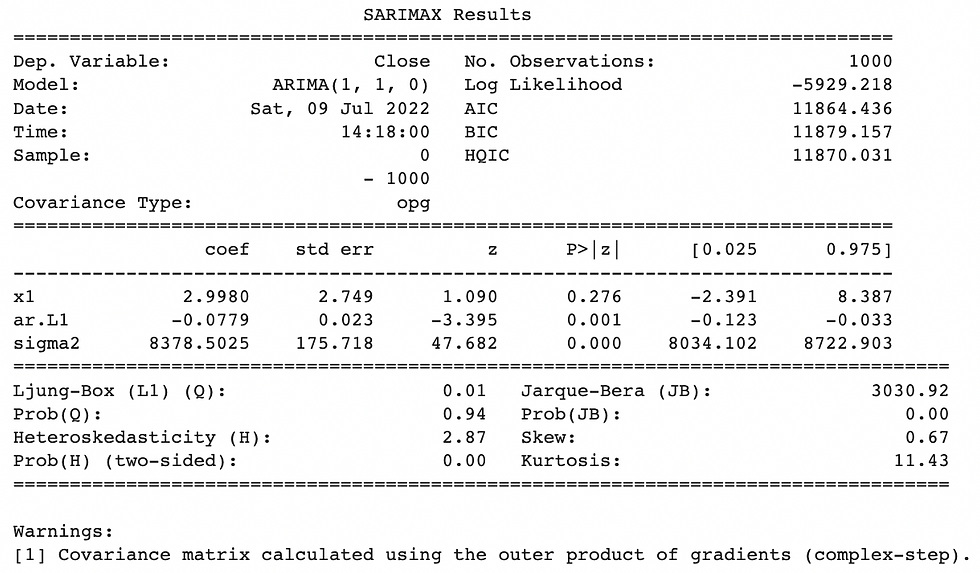

It turns out that from the results obtained, both ARIMA(0,1,1) and ARIMA(1,1,0) produce significant coefficients in the model. This can be seen from the confidence interval for each coefficient that does not contain a value of 0.

From the two models, the final model will be selected by looking at the AIC value of each model. The model with the smallest AIC value is the model that has the better performance. So the model with the smallest AIC is ARIMA(0,1,1) and this becomes the final model.

Forecasting

The next step is to predict the test data and forecast for the next 100 days. Plot results of prediction and forecasting data.

#Prediction
prediction_arima = result1.get_prediction(start=1, end=len(df))
pred = prediction_arima.predicted_mean

pred_df = pd.DataFrame(pred.values, columns=['pred']).join(df['Date'])

#Forecast Next 100 Days
n_forecast = 100

forecast_arima = result1.get_forecast(steps=n_forecast)

yhat = forecast_arima.predicted_mean
yhat_conf_int = forecast_arima.conf_int(alpha=0.05)

yhat_date = pd.DataFrame(pd.date_range(start = '2022-07-01', periods = 100, freq='B'), columns=['Date'])

yhat_df = pd.DataFrame(yhat.values,  columns=['yhat']).join(yhat_date)

# Result Forecastyhat_df

lower_series = pd.DataFrame(yhat_conf_int['lower Close'].values, columns=['lower']).join(yhat_date)
upper_series = pd.DataFrame(yhat_conf_int['upper Close'].values, columns=['upper']).join(yhat_date)

pio.templates.default = "plotly_white"

st_fig = go.Figure()

st_fig.add_trace(go.Scatter(x = train['Date'], y = train['Close'], mode = 'lines', name = 'Train'))
st_fig.add_trace(go.Scatter(x = test['Date'], y = test['Close'], mode = 'lines', name= 'Test'))

st_fig.add_trace(go.Scatter(x = pred_df['Date'], y = pred_df['pred'],
                     line = dict(color='firebrick', width=2, dash='dot'), name= 'Prediction'))
st_fig.add_trace(go.Scatter(x = yhat_df['Date'], y = yhat_df['yhat'],
                     line = dict(color='firebrick', width=2, dash='dot'), name= 'Forecasting'))

st_fig.add_traces(go.Scatter(x=lower_series['Date'], y = lower_series['lower'],
                    line = dict(color='#d5dbd6'), name='lower'))
st_fig.add_traces(go.Scatter(x=upper_series['Date'], y = upper_series['upper'],
                    line = dict(color='#d5dbd6'),fill='tonexty', name='upper'))

st_fig.update_layout(title='ARIMA (0,1,1)')
st_fig.show()

Evaluation

Next, evaluate the model based on the prediction results on the test data and the actual test data using the RMSE (Root Mean Squared Error) metric.

rmse_arima =  mean_squared_error(test['Close'], pred_df['pred'][split_time:], squared=False)
rmse_arima

310.2014399308559

Long Short Term Memory (LSTM)

Next, we will use deep learning methods for analysis. In general, the use of deep learning methods uses a neural network model. One of the neural network models used to train sequential data types is the Recurrent Neural Network (RNN). In its development, RNN has a drawback that the model cannot predict data based on information that has been stored for a long time. Thus, LSTM is present as a modification of the RNN model to complete these shortcomings. The LSTM model is able to remember data/information that has been stored for a long time and delete irrelevant data/information for further use.

In general, the Neural network model trains data as supervised learning, meaning that the model requires predictors data and target data. However, the problem is in time series data, it does not have predictors and target components. So we need to modify the data, next we will introduce the concept of window size.

Window size is the number of features (predictors) that will be used to predict the target. In other words, numbers from the previous time data are used to predict the next day. For example, if we specify window size = 2, then to predict tomorrow (target) we need today's and yesterday's data (predictors). Suppose we have time series data as follows: [1,2,3,4,5,6,7,8,9] Next, we choose window size = 5, then the required data format is as follows:

[1,2,3,4,5][6]

[2,3,4,5,6][7]

[3,4,5,6,7][8]

[4,5,6,7,8][9]

To prepare data in the required format, we can use the Tensorflow module, namely TimeseriesGenerator.

# Prepare Dataset

scaler = StandardScaler()
train_scale = pd.DataFrame(scaler.fit_transform(np.array(train['Close']).reshape(-1,1)), columns=['Close'])
train_scale_df = train[['Date']].join(train_scale)

test_scale = pd.DataFrame(scaler.transform(np.array(test['Close']).reshape(-1,1)), index=test.index, columns=['Close'])
test_scale_df = test[['Date']].join(test_scale)

window_size=10

train_generator = TimeseriesGenerator(train_scale_df['Close'].to_numpy(),
                                      train_scale_df['Close'].to_numpy(),length=window_size, batch_size=28)
test_generator = TimeseriesGenerator(test_scale_df['Close'].to_numpy(),
                                     test_scale_df['Close'].to_numpy(), length=window_size, batch_size=1)

Modeling

# Modeling
model = tf.keras.models.Sequential([tf.keras.layers.LSTM(100, input_shape=(window_size,1), return_sequences=True),
     tf.keras.layers.LSTM(50, return_sequences=True),
     tf.keras.layers.LSTM(10),
     tf.keras.layers.Dense(64, activation='relu'),
     tf.keras.layers.Dense(16, activation='relu'),
     tf.keras.layers.Dense(1)])
     
model.compile(loss='mse',optimizer=tf.keras.optimizers.Adam(),metrics=['mape'])
history = model.fit(train_generator,epochs=100)

Epoch 1/100 36/36 [==============================] - 16s 50ms/step - loss: 0.7779 - mape: 151.6860 Epoch 2/100 36/36 [==============================] - 2s 46ms/step - loss: 0.2504 - mape: 234.0566 Epoch 3/100 36/36 [==============================] - 2s 45ms/step - loss: 0.1512 - mape: 206.7620 Epoch 4/100 36/36 [==============================] - 2s 45ms/step - loss: 0.1184 - mape: 151.3236 Epoch 5/100 36/36 [==============================] - 2s 43ms/step - loss: 0.0792 - mape: 131.0709 Epoch 6/100 36/36 [==============================] - 2s 49ms/step - loss: 0.0595 - mape: 109.3048 Epoch 7/100 36/36 [==============================] - 1s 38ms/step - loss: 0.0735 - mape: 131.0346 Epoch 8/100 36/36 [==============================] - 1s 39ms/step - loss: 0.0679 - mape: 139.2482 Epoch 9/100 36/36 [==============================] - 1s 41ms/step - loss: 0.0481 - mape: 117.4105 Epoch 10/100 36/36 [==============================] - 2s 44ms/step - loss: 0.0578 - mape: 94.5498 Epoch 11/100 36/36 [==============================] - 1s 31ms/step - loss: 0.0689 - mape: 116.0270 Epoch 12/100 36/36 [==============================] - 1s 23ms/step - loss: 0.0665 - mape: 148.1262 Epoch 13/100 36/36 [==============================] - 1s 23ms/step - loss: 0.0414 - mape: 98.3992 Epoch 14/100 36/36 [==============================] - 1s 22ms/step - loss: 0.0471 - mape: 114.8499 Epoch 15/100 36/36 [==============================] - 1s 22ms/step - loss: 0.0454 - mape: 82.2728 Epoch 16/100 36/36 [==============================] - 1s 23ms/step - loss: 0.0351 - mape: 76.8623 Epoch 17/100 36/36 [==============================] - 1s 23ms/step - loss: 0.0361 - mape: 72.3177 Epoch 18/100 36/36 [==============================] - 1s 23ms/step - loss: 0.0356 - mape: 84.9144 Epoch 19/100 36/36 [==============================] - 1s 22ms/step - loss: 0.0308 - mape: 69.3175 Epoch 20/100 36/36 [==============================] - 1s 23ms/step - loss: 0.0301 - mape: 78.5911 Epoch 21/100 36/36 [==============================] - 1s 24ms/step - loss: 0.0310 - mape: 73.9265 Epoch 22/100 36/36 [==============================] - 1s 23ms/step - loss: 0.0352 - mape: 76.4437 Epoch 23/100 36/36 [==============================] - 1s 23ms/step - loss: 0.0297 - mape: 74.6303 Epoch 24/100 36/36 [==============================] - 1s 23ms/step - loss: 0.0305 - mape: 85.8269 Epoch 25/100 36/36 [==============================] - 1s 23ms/step - loss: 0.0256 - mape: 73.4911 Epoch 26/100 36/36 [==============================] - 1s 22ms/step - loss: 0.0260 - mape: 74.2237 Epoch 27/100 36/36 [==============================] - 1s 22ms/step - loss: 0.0257 - mape: 83.6110 Epoch 28/100 36/36 [==============================] - 1s 22ms/step - loss: 0.0297 - mape: 89.1856 Epoch 29/100 36/36 [==============================] - 1s 23ms/step - loss: 0.0277 - mape: 71.9880 Epoch 30/100 36/36 [==============================] - 1s 23ms/step - loss: 0.0338 - mape: 71.7688 Epoch 31/100 36/36 [==============================] - 1s 22ms/step - loss: 0.0232 - mape: 73.2884 Epoch 32/100 36/36 [==============================] - 1s 23ms/step - loss: 0.0244 - mape: 72.7978 Epoch 33/100 36/36 [==============================] - 1s 22ms/step - loss: 0.0237 - mape: 70.1510 Epoch 34/100 36/36 [==============================] - 1s 23ms/step - loss: 0.0207 - mape: 74.2790 Epoch 35/100 36/36 [==============================] - 1s 23ms/step - loss: 0.0207 - mape: 61.9844 Epoch 36/100 36/36 [==============================] - 1s 23ms/step - loss: 0.0229 - mape: 77.2031 Epoch 37/100 36/36 [==============================] - 1s 23ms/step - loss: 0.0217 - mape: 65.7867 Epoch 38/100 36/36 [==============================] - 1s 22ms/step - loss: 0.0197 - mape: 65.7314 Epoch 39/100 36/36 [==============================] - 1s 22ms/step - loss: 0.0226 - mape: 73.9430 Epoch 40/100 36/36 [==============================] - 1s 23ms/step - loss: 0.0210 - mape: 65.8813 Epoch 41/100 36/36 [==============================] - 1s 22ms/step - loss: 0.0239 - mape: 70.1129 Epoch 42/100 36/36 [==============================] - 1s 22ms/step - loss: 0.0242 - mape: 80.0181 Epoch 43/100 36/36 [==============================] - 1s 24ms/step - loss: 0.0182 - mape: 64.4561 Epoch 44/100 36/36 [==============================] - 1s 24ms/step - loss: 0.0164 - mape: 57.8481 Epoch 45/100 36/36 [==============================] - 1s 23ms/step - loss: 0.0162 - mape: 59.9344 Epoch 46/100 36/36 [==============================] - 1s 23ms/step - loss: 0.0172 - mape: 62.4360 Epoch 47/100 36/36 [==============================] - 1s 24ms/step - loss: 0.0189 - mape: 57.1534 Epoch 48/100 36/36 [==============================] - 1s 23ms/step - loss: 0.0181 - mape: 57.8078 Epoch 49/100 36/36 [==============================] - 1s 23ms/step - loss: 0.0216 - mape: 80.9789 Epoch 50/100 36/36 [==============================] - 1s 23ms/step - loss: 0.0201 - mape: 58.1512 Epoch 51/100 36/36 [==============================] - 1s 23ms/step - loss: 0.0161 - mape: 61.3567 Epoch 52/100 36/36 [==============================] - 1s 23ms/step - loss: 0.0148 - mape: 52.7492 Epoch 53/100 36/36 [==============================] - 1s 23ms/step - loss: 0.0171 - mape: 53.3641 Epoch 54/100 36/36 [==============================] - 1s 24ms/step - loss: 0.0150 - mape: 54.2902 Epoch 55/100 36/36 [==============================] - 1s 24ms/step - loss: 0.0197 - mape: 61.8509 Epoch 56/100 36/36 [==============================] - 1s 23ms/step - loss: 0.0281 - mape: 67.6075 Epoch 57/100 36/36 [==============================] - 1s 24ms/step - loss: 0.0204 - mape: 69.4066 Epoch 58/100 36/36 [==============================] - 1s 22ms/step - loss: 0.0212 - mape: 62.5444 Epoch 59/100 36/36 [==============================] - 1s 22ms/step - loss: 0.0159 - mape: 53.6175 Epoch 60/100 36/36 [==============================] - 1s 23ms/step - loss: 0.0213 - mape: 54.8912 Epoch 61/100 36/36 [==============================] - 1s 23ms/step - loss: 0.0179 - mape: 68.3458 Epoch 62/100 36/36 [==============================] - 1s 23ms/step - loss: 0.0153 - mape: 54.0348 Epoch 63/100 36/36 [==============================] - 1s 22ms/step - loss: 0.0152 - mape: 58.4095 Epoch 64/100 36/36 [==============================] - 1s 22ms/step - loss: 0.0136 - mape: 49.1435 Epoch 65/100 36/36 [==============================] - 1s 23ms/step - loss: 0.0149 - mape: 51.1637 Epoch 66/100 36/36 [==============================] - 1s 23ms/step - loss: 0.0170 - mape: 47.8374 Epoch 67/100 36/36 [==============================] - 1s 23ms/step - loss: 0.0158 - mape: 45.6699 Epoch 68/100 36/36 [==============================] - 1s 23ms/step - loss: 0.0126 - mape: 45.2688 Epoch 69/100 36/36 [==============================] - 1s 23ms/step - loss: 0.0134 - mape: 53.1309 Epoch 70/100 36/36 [==============================] - 1s 23ms/step - loss: 0.0133 - mape: 46.3962 Epoch 71/100 36/36 [==============================] - 1s 23ms/step - loss: 0.0149 - mape: 54.0003 Epoch 72/100 36/36 [==============================] - 1s 23ms/step - loss: 0.0129 - mape: 46.0470 Epoch 73/100 36/36 [==============================] - 1s 23ms/step - loss: 0.0131 - mape: 50.0148 Epoch 74/100 36/36 [==============================] - 1s 23ms/step - loss: 0.0139 - mape: 45.4035 Epoch 75/100 36/36 [==============================] - 1s 22ms/step - loss: 0.0139 - mape: 50.2443 Epoch 76/100 36/36 [==============================] - 1s 23ms/step - loss: 0.0118 - mape: 46.7176 Epoch 77/100 36/36 [==============================] - 1s 22ms/step - loss: 0.0126 - mape: 47.4992 Epoch 78/100 36/36 [==============================] - 1s 23ms/step - loss: 0.0143 - mape: 49.3194 Epoch 79/100 36/36 [==============================] - 1s 22ms/step - loss: 0.0126 - mape: 48.3135 Epoch 80/100 36/36 [==============================] - 1s 22ms/step - loss: 0.0126 - mape: 52.5428 Epoch 81/100 36/36 [==============================] - 1s 25ms/step - loss: 0.0144 - mape: 43.7217 Epoch 82/100 36/36 [==============================] - 1s 23ms/step - loss: 0.0131 - mape: 47.8618 Epoch 83/100 36/36 [==============================] - 2s 51ms/step - loss: 0.0117 - mape: 48.1736 Epoch 84/100 36/36 [==============================] - 1s 23ms/step - loss: 0.0120 - mape: 45.2521 Epoch 85/100 36/36 [==============================] - 1s 23ms/step - loss: 0.0138 - mape: 49.6291 Epoch 86/100 36/36 [==============================] - 1s 24ms/step - loss: 0.0155 - mape: 52.0540 Epoch 87/100 36/36 [==============================] - 1s 23ms/step - loss: 0.0130 - mape: 44.7114 Epoch 88/100 36/36 [==============================] - 1s 23ms/step - loss: 0.0130 - mape: 43.8167 Epoch 89/100 36/36 [==============================] - 1s 23ms/step - loss: 0.0128 - mape: 54.2421 Epoch 90/100 36/36 [==============================] - 1s 25ms/step - loss: 0.0141 - mape: 46.6386 Epoch 91/100 36/36 [==============================] - 2s 42ms/step - loss: 0.0147 - mape: 50.5105 Epoch 92/100 36/36 [==============================] - 1s 24ms/step - loss: 0.0130 - mape: 51.9115 Epoch 93/100 36/36 [==============================] - 1s 24ms/step - loss: 0.0167 - mape: 52.0781 Epoch 94/100 36/36 [==============================] - 1s 23ms/step - loss: 0.0238 - mape: 52.1075 Epoch 95/100 36/36 [==============================] - 1s 24ms/step - loss: 0.0160 - mape: 53.3588 Epoch 96/100 36/36 [==============================] - 1s 23ms/step - loss: 0.0133 - mape: 48.6066 Epoch 97/100 36/36 [==============================] - 1s 23ms/step - loss: 0.0128 - mape: 46.3881 Epoch 98/100 36/36 [==============================] - 1s 24ms/step - loss: 0.0117 - mape: 45.5153 Epoch 99/100 36/36 [==============================] - 1s 22ms/step - loss: 0.0118 - mape: 43.7350 Epoch 100/100 36/36 [==============================] - 1s 23ms/step - loss: 0.0122 - mape: 48.5110

plt.figure(figsize=(8,5))

loss = history.history['loss']
epochs = range(1, len(loss) + 1)

plt.plot(epochs, loss)
plt.title('Training loss')
plt.show()

#Prediction

train_predict = model.predict(train_generator)
train_predict = pd.DataFrame(scaler.inverse_transform(train_predict.reshape(-1,1)), columns=['Close'])

test_predict = model.predict(test_generator)
test_predict = pd.DataFrame(scaler.inverse_transform(test_predict.reshape(-1,1)), columns=['Close'])

pio.templates.default = "plotly_white"

st_fig = go.Figure()

st_fig.add_trace(go.Scatter(x = train['Date'], y = train['Close'], mode = 'lines', name = 'Train'))
st_fig.add_trace(go.Scatter(x = test['Date'], y = test['Close'], mode = 'lines', name= 'Test'))

st_fig.add_trace(go.Scatter(x = train['Date'][10:], y = train_predict['Close'],
                 line = dict(color='#5d05f5', width=2, dash='dot'), name= 'Train Prediction'))
st_fig.add_trace(go.Scatter(x = test['Date'][10:], y = test_predict['Close'],
                 line = dict(color='#5d05f5', width=2, dash='dot'), name= 'Test Prediction'))

st_fig.update_layout(title='LSTM')
st_fig.show()

Forecasting

The next step is to forecast for the next 100 days. Plot results of forecasting data.

# Forcasting
def predict(num_prediction, model):
    prediction_list = test_scale['Close'].to_numpy()[-window_size:]
    
    for _ in range(num_prediction):
      x = prediction_list[-window_size:]
      x = x.reshape(1, window_size, 1)
      out = model.predict(x)
      prediction_list = np.append(prediction_list, out)
      
    forecast = prediction_list[window_size:]
    forecast = pd.DataFrame(scaler.inverse_transform(forecast.reshape(-1,1)), columns=['Close'])
    forecast['Date'] = pd.date_range(start = test['Date'].to_list()[-1] + pd.DateOffset(days=1), periods = num_prediction, freq='B')
    
    return forecast

forecast_lstm = predict(100, model)

# Result Forecast
forecast_lstm

pio.templates.default = "plotly_white"

st_fig = go.Figure()

st_fig.add_trace(go.Scatter(x = train['Date'], y = train['Close'], mode = 'lines', name = 'Train'))
st_fig.add_trace(go.Scatter(x = test['Date'], y = test['Close'], mode = 'lines', name= 'Test'))

st_fig.add_trace(go.Scatter(x = train['Date'][10:], y = train_predict['Close'],
                            line = dict(color='#5d05f5', width=2, dash='dot'), name= 'Train Prediction'))
   
st_fig.add_trace(go.Scatter(x = test['Date'][10:], y = test_predict['Close'],
                            line = dict(color='#5d05f5', width=2, dash='dot'), name= 'Test Prediction'))
   
st_fig.add_trace(go.Scatter(x = forecast_lstm['Date'], y = forecast_lstm['Close'],
                            line = dict(color='#5d05f5', width=2, dash='dot'), name= 'Forecast'))
   
st_fig.update_layout(title='LSTM + Forecast')
st_fig.show()

Evaluation

Next, evaluate the model based on the prediction results on the test data and the actual test data using the RMSE (Root Mean Squared Error) metric.

rmse_lstm =  mean_squared_error(test['Close'][10:], test_predict['Close'], squared=False)
rmse_lstm

165.56844464497928

FB Prophet Model

In addition to the above models, there is a popular forecasting model used, namely the FB Prophet. Prophet is open-source software released by Facebook's Core Data Science team in 2017. Prophet model is based on an additive model where non-linear trends are fit with yearly, weekly, and daily seasonality, plus holiday effects.

To use this model, we need to prepare the data according to the required format. Where the data must consist of columns ds (datesamp) and y (observation). It should be noted that the column naming must also match the format, and for ds the format used is YYYY-MM-DD. Ok, Let's prepare the data!

train_fp = pd.DataFrame({'ds' : train['Date'], 'y' : train['Close']})
train_fp.head()

Modeling Then do the modeling, because our data is in the form of daily, we set daily_seasonality=True.

model_fp = Prophet(daily_seasonality=True)
model_fp.fit(train_fp)

<prophet.forecaster.Prophet at 0x7fec536eb3d0>

Forecasting Then do forecasting for test data and the next 100 days and plot the results.

future = model_fp.make_future_dataframe(periods=len(test)+100, freq='B')
future.tail()

forecast = model_fp.predict(future)
forecast[['ds', 'yhat', 'yhat_lower', 'yhat_upper']].tail()

pio.templates.default = "plotly_white"

st_fig = go.Figure()

st_fig.add_traces(go.Scatter(x=forecast['ds'], y = forecast['yhat_lower'],
                          line = dict(color='#d5dbd6'), name='lower'))
st_fig.add_traces(go.Scatter(x=forecast['ds'], y = forecast['yhat_upper'],
                          line = dict(color='#d5dbd6'),
                fill='tonexty', name='upper'))

st_fig.add_trace(go.Scatter(x = train['Date'], y = train['Close'], mode = 'lines', name = 'Train'))
st_fig.add_trace(go.Scatter(x = test['Date'], y = test['Close'], mode = 'lines', name= 'Test'))

st_fig.add_trace(go.Scatter(x = forecast['ds'], y = forecast['yhat'],
                            line = dict(color='green', width=2, dash='dot'), name= 'Forecasting'))

st_fig.update_layout(title='FB Prophet')
st_fig.show()

In addition, Prophet also provides its own function to plot forecast results as follows:

model_fp.plot(forecast)
plt.title('FB Prophet')
plt.show()

Evaluation Next, evaluate the model based on the prediction results of the test data and the actual test data using the RMSE (Root Mean Squared Error) metric.

rmse_fp =  mean_squared_error(test['Close'], forecast['yhat'][split_time:split_time+len(test)], squared=False)

rmse_fp

411.4355078446341

Summary

pd.DataFrame({'Model' : ['ARIMA', 'LSTM', 'FB Prophet'],'RMSE Test Set': [rmse_arima, rmse_lstm, rmse_fp]})

That's all our hands-on for time series analysis, especially for univariate time series. The writing on this blog is certainly not perfect and there may still have deficiencies.

Of course, I'm also still in the learning stage, thank you for reading, I hope it's useful, I'd love it if you comment for any suggestions and hopefully, we can learn together. You can also be connected with me on LinkedIn ^^.